6 Mixed and Behavioral Strategies
%if doesn’t work
%random variable %random vector or matrix%differentiated vector or matrix
%#TODO%#TODO
% Basic notation - general % Basic notation - general % Special symbols % Basic functions %image %cardinality % Operators - Analysis % Linear algebra % Linear algebra - Matrices % Statistics %at time % Useful commands % Game Theory %T-stage game %strategy in a repeated game %successor function %player function%action function
% Optimization$$
6.1 Introduction
Assume two players and a finite extensive-form game \(G\)
Definition 6.1 A mixed strategy \(\sigma_i\) of player \(i\) in \(G\) is a mixed strategy of player \(i\) in the corresponding strategic-form game.
In other words, a mixed strategy \(\sigma_i\) in \(G\) is a probability distribution of \(S_i\) (recall that \(S_i\) is the set of all pure strategies, i.e. functions of the form \(s_i : H_i \to A\)). As before, we denote by \(\Sigma_i\) the set of all mixed strategies of player \(i\).
Definition 6.2 A behavioral (mixed) strategy of player \(i\) in \(G\) is a function \(\beta_i : H_i \to \Delta(A)\) such that for every \(h \in H_i\) and every \(a \in A\): \(\beta_i(h)(a) = 0\) if \(a \not\in \chi(h)\).
For mixed strategy, we randomize once for our behaviors everywhere, which we then follow deterministically.
On the other hand, for the behavioral strategies we randomize for each choice of the action we take.
Given a profile \(\boldsymbol{\beta }= (\beta_1, \beta_2)\) of behavioral strategies, we denote by \(P_{\boldsymbol{\beta}}(z)\) the probability of reaching \(z \in Z\) when \(\boldsymbol{\beta}\) is used, i.e., \[ P_{\boldsymbol{\beta}}(z) = \prod_{l = 1}^k \beta_{\rho(h_{l-1})}(h_{l-1})(a_l), \] where \(h_0 a_1 h_1 a_2 h_2 \dots a_k h_k\) is the unique path from \(h_0\) to \(h_k = z\). We also define the expected payoff under the behavioral strategy \(\boldsymbol{\beta}\) as \(u_i(\boldsymbol{\beta}) := \sum_{z \in Z} P_{\boldsymbol{\beta}(z)} u_i(z)\).
6.2 Examples
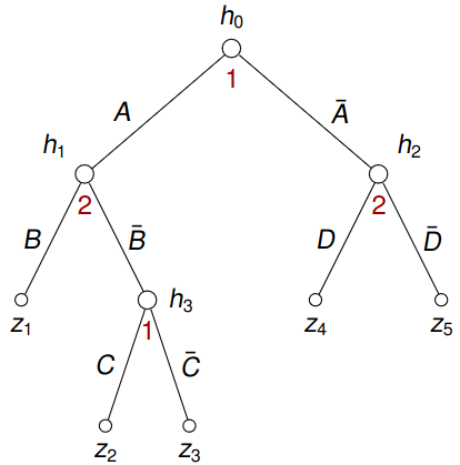
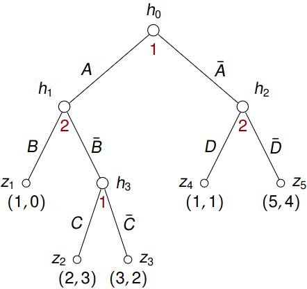
Example 6.1 Consider a game given by a tree in Figure 6.1.

Then pure strategies of player 1 are \(AC, A\bar C, \bar A C, \bar A \bar C\) and an example of a mixed strategy \(\sigma_1\) of player 1 might be: \[ \sigma_1(AC) = \frac 1 3, \sigma_1(A \bar C) = \frac 1 9, \sigma_1(\bar A C) = \frac 1 6, \sigma_1(\bar A \bar C) = \frac {11} {18}. \]
On the other hand, an example of behavioral strategies of both players can be:
- player 1: \(\beta_1(h_0)(A) =\frac 1 3\) and \(\beta_1(h_3)(C) = \frac 1 2\);
- player 2: \(\beta_2(h_1)(B) = \frac 1 4\) and \(\beta_2(h_2)(D) = \frac 1 5\).
Then for example \(P_{(\beta_1, \beta_2)}(z_2) = \frac 1 3 \left( 1 - \frac 1 4 \right)\frac 1 2 = \frac 1 8\).

After assigning payoffs, see Figure 6.2, we can compute expected payoff of the behavioral strategy \(\boldsymbol{\beta}\): \[\begin{align*} u_1(\boldsymbol{\beta}) &= P_{\boldsymbol{\beta}} (z_1) \cdot 1 + P_{\boldsymbol{\beta}} (z_2) \cdot 2 + P_{\boldsymbol{\beta}} (z_3) \cdot 3 + P_{\boldsymbol{\beta}} (z_4) \cdot 1 + P_{\boldsymbol{\beta}} (z_5) \cdot 5 \\ &= \frac 1 3 \frac 1 4 1 + \frac 1 3 \frac 3 4 \frac 1 2 2 + \frac 1 3 \frac 3 4 \frac 1 2 3 + \frac 2 3 \frac 1 5 1 + \frac 2 3 \frac 4 5 5 \approx 3.508. \end{align*}\]
Each pure strategy can be seen as a behavioral strategy. Consider e.g. \(s_1 : H_1 \to A\) defined by \(s_1 (h_0) = A\) and \(s_1 (h_3) = C\). The corresponding behavioral strategy \(\beta_1\) would satisfy \(\beta_1(h_0)(A) = \beta_1 (h_3)(C) = 1\) (i.e. select actions chosen by \(s_1\) with probability 1). Now given a behavioral strategy \(\beta_2\) of player 2 defined by \(\beta_2(h_1)(B) = \frac 1 4\) and \(\beta_2(h_2)(D) = \frac 1 5\) we obtain \[ P_{(s_1, \beta_2)}(z_2) = P_{(\beta_1, \beta_2)}(z_2) = 1 \left( 1 - \frac 1 4 \right)1 = \frac 3 4. \]
6.3 Equivalence
Let \(\boldsymbol{\alpha }= (\alpha_1, \alpha_2)\) be a strategy profile where each \(\alpha_i\) is either mixed or behavioral.
The game is then played as follows:
- if \(\alpha_1\) is mixed, select randomly a pure strategy \(\beta_1\) according to \(\alpha_1\), else \(\beta_1 := \alpha_1\);
- if \(\alpha_2\) is mixed, select randomly a pure strategy \(\beta_2\) according to \(\alpha_2\), else \(\beta_2 := \alpha_2\);
- play \((\beta_1, \beta_2)\) and collect payoffs.
Denote the resulting payoffs by \(u_1(\boldsymbol{\alpha})\) and \(u_2(\boldsymbol{\alpha})\).
Lemma 6.1 For every mixed/behavioral strategy \(\alpha_1\) of player 1 there is a behavioral/mixed strategy \(\alpha'_1\) such that for every mixed/behavioral strategy \(\alpha_2\) we have that \(u_i(\alpha_1, \alpha_2) = u_i(\alpha'_1, \alpha_2)\) for \(i \in \left\{1, 2\right\}\).
Example 6.2 Consider the following game:
Let us first focus on “converting” behavioral strategies to mixed ones. Let \(\boldsymbol{\alpha }= (\alpha_1, \alpha_2)\) be a behavioral strategy profile, that is
- \(\alpha_1(h_0)(A) = p\) and \(\alpha_1(h_2)(C) = q\);
- \(\alpha_2(h_1)(U) = u\).
Then the equivalent mixed strategy \(\alpha_1'\) of player 1 is: \[\begin{align*} \alpha_1'(AC) & = pq, & \alpha_1'(AD) & = p(1 - q), \\ \alpha_1'(BC) & = (1-p)q, & \alpha_1'(BD) & = (1-p)(1 - q), \end{align*}\] because \[ P_{(\alpha_1, \alpha_2)} (z_2) = (1 - p)u = (\overbrace{(1 - p)q}^{\alpha_1'(BC)} + \overbrace{(1 - p)(1 - q)}^{\alpha_1'(BD)}) \cdot u = P_{(\alpha_1', \alpha_2)}(z_2) \] and similarly for the other terminal nodes.
Let us now turn our attention to “converting” mixed strategies to behavioral ones. Let \(\alpha_1\) be a mixed strategy of player 1: \[\begin{align*} \alpha_1(AC) & = e_{AC}, & \alpha_1(AD) & = e_{AD}, \\ \alpha_1(BC) & = e_{BC}, & \alpha_1(BD) & = e_{BD}. \end{align*}\]
Then we can construct an equivalent behavioral strategy \(\alpha_1'\) as \[\begin{align*} \alpha_1'(h_0)(A) & = e_{AC} + e_{AD}, & \alpha_1'(h_0)(B) & = e_{BC} + e_{BD}, \\ \alpha_1'(h_2)(C) & = \frac {e_{BC}}{e_{BC} + e_{BD}}, & \alpha_1'(h_2)(D) & = \frac {e_{BD}}{e_{BC} + e_{BD}}, \end{align*}\] where \(\frac {e_{BC}}{e_{BC} + e_{BD}}\) can be interpreted as a conditional probability \(P(C| BC \cup BD)\). We can then check our calculation: \[ P_{(\alpha_1, \alpha_2)}(z_3) = e_{BC} \cdot (1 - u) = \overbrace{(e_{BC} + e_{BD})}^{\alpha_1'(h_0){B}} \cdot \overbrace{\frac {e_{BC}} {e_{BC} + e_{BD}}}^{\alpha_1'(h_2)(C)} \cdot (1 - u) = P_{(\alpha_1', \alpha_2)}(z_3) \]