5 Extensive Form Games

Static games (modeled using strategic-form games) cannot capture games that unfold over time. In particular, as all players move simultaneously, there is no way to model situations in which the order of moves is important. Imagine e.g. chess where players take turns, in every round, a player knows all turns of the opponent before making his own turn. There are many examples of dynamic games: markets that change over time, political negotiations, models of computer systems, etc.

We model dynamic games using extensive-form games, a tree-like model that allows us to express the sequential nature of games. We start with perfect information games, where each player always knows the results of all previous moves. Then generalize to imperfect information, where players may have only partial knowledge of these results (e.g. most card games).

Example 5.1 Consider a game:

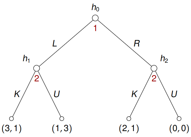
Here $h_0, h_1, h_2$ are non-terminal nodes, leaves are terminal nodes. Each non-terminal node is owned by a player who chooses an action, e.g. $h_1$ is owned by player 2 who chooses either $K$ or $U$. Every action results in a transition to a new node, so choosing $L$ in $h_0$ results in a move to $h_1$. When a play reaches a terminal node, players collect payoffs, e.g. the leftmost terminal node gives 3 to player 1 and 1 to player 2.

5.1 Basic Concepts

Definition 5.1 A perfect-information extensive-form game is a tuple $G = (N,A,H,Z,\chi,\rho,\pi,h_0, \boldsymbol{u})$ where

$N = \left\{1, \dots, n\right\}$ is a set of $n$ players, $A$ is a (single) set of actions;
$H$ is a set of non-terminal (choices) nodes, $Z$ is a set of terminal nodes (assume $Z \cap H = \emptyset$), denote $\mathcal{H} = H \cup Z$;
$\chi: H \to (2^A \setminus \left\{\emptyset\right\})$ is the action function, which assigns to each non-terminal choice node a non-empty set of enabled actions;
$\rho: H \to N$ is the player function, which assigns to each non-terminal node a player $i$ who chooses an action there, we define $H_i := \left\{h \in H | \rho(h) = i\right\}$;
$\pi: H \times A \to \mathcal{H}$ is the successor function, which maps a non-terminal node and an action to a new node, such that
- $h_0$ is the only node that is not in the image of $\pi$ (i.e. nothing maps to the root);
- for all $h_1, h_2 \in H$ and for all $a_1 \in \chi(h_1)$ and all $a_2 \in \chi(h_2)$, if $\pi(h_1,a_1) = \pi(h_2, a_2)$, then $h_1 = h_2$ and $a_1 = a_2$;
$\boldsymbol{u} = (u_1, \dots, u_n)$, where each $u_i : Z \to \mathbb{R}$ is a payoff function for player $i$ in the terminal nodes of $Z$.

We say that $h'$ is a child of $h$, and $h$ is a parent of $h'$ if there is $a \in \chi(h)$ such that $h' = \pi(h, a)$. A path from $h \in H$ to $h' \in H$ is a sequence $h_1 a_2 h_2 a_3 h_3 \dots h_{k-1} a_k h_k$ where $h_1 = h, h_k = h'$ and $\pi(h_{j−1}, a_j) = h_j$ for every $1 < j \leq k$.

Note

Note that, in particular, $h$ is a path from $h$ to $h$.

Also, $h' \in \mathcal{H}$ is reachable from $h \in \mathcal{H}$ if there is a path from $h$ to $h'$.

Note

If $h'$ is reachable from $h$, we say that $h'$ is a descendant of $h$ and $h$ is an ancestor of $h'$.

Every perfect-information extensive-form game can be seen as a game on a rooted tree $(\mathcal{H}, E, h_0)$ where

$\mathcal{H} = H \cup Z$ is a set of nodes,
$E \subseteq \mathcal{H} \times \mathcal{H}$ is a set of edges defined by $(h, h') \in E$ iff $h \in H$ and there is a $a \in \chi(h)$ such that $\pi(h, a) = h'$,
$h_0$ is the root.

Example 5.2 Consider a game

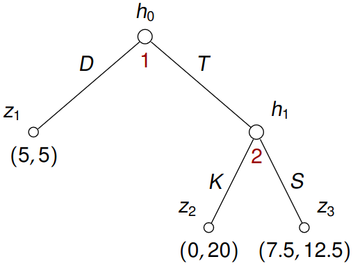
Two players, both start with 5$ and player 2 is a broker who wants to “help” player 1. Player 1 either distrusts (D) player 2 and keeps the money (payoffs (5, 5)), or trusts (T) player 2 and passes 5$ to player 2. If player 1 chooses to trust player 2, the total money (10) is doubled by the experimenter in the hands of player 2. Player 2 may either keep (K) the additional 15$ (resulting in (0, 20)), or share (S) it with player 1 (resulting in (7.5, 12.5)).

Let us put $N = \left\{1,2\right\}, A = \left\{D, T, K, S\right\}$, $H = \left\{h_0, h_1\right\}$ and $Z = \left\{z_1, z_2, z_3\right\}$. Moreover \[ \begin{gathered} \chi(h_0) = \left\{D,T\right\}, \quad \chi(h_1) = \left\{S,K\right\} \end{gathered} \] and $\rho(h_0) = 1$, $\rho(h_1) = 2$ with \[ \pi(h_0, D) = z_1, \quad \pi(h_0, T) = h_1, \quad \pi(h_1, K) = z_2, \quad \pi(h_1, S) = z_3 \] and lastly \[ \boldsymbol{u}(z_1) = (5, 5), \quad \boldsymbol{u}(z_2) = (0, 20), \quad \boldsymbol{u}(z_3) = (7.5, 12.5). \]

Example 5.3 (Stackelberg Competition) Very similar to Cournot duopoly, this time we have two identical firms, players 1 and 2, produce some good. Denote by $q_1$ and $q_2$ quantities produced by firms 1 and 2, resp. The total quantity of products in the market is $q_1 + q_2$. The price of each item is $\kappa − q_1 − q_2$ where $\kappa > 0$ is fixed. Firms have a common per-item production cost $c$.

As opposed to Cournot duopoly, firm 1 moves first, and chooses the quantity $q_1 \in [0, \infty)$. Afterward, the firm 2 chooses $q_2 \in [0, \infty)$ (knowing $q_1$) and then the firms get their payoffs.

As an extensive-form game, we get \[ \begin{gathered} N = \left\{1,2\right\}, \quad A = [0, \infty), \\ H = \left\{h_0, h_1^{q_1} | q_1 \in [0, \infty)\right\}, \quad Z = \left\{z^{q_1, q_2} | q_1, q_2 \in [0, \infty)\right\}, \\ \chi(h_0) = [0, \infty), \quad \chi(h_1^{q_1}) = [0, \infty), \quad \rho(h_0) = 1, \quad \rho(h_1^{q_1}) = 2, \\ \pi(h_0, q_1) = h_1^{q_1}, \quad \pi(h_1^{q_1}, q_2) = z_{q_1, q_2}, \\ \boldsymbol{u}(z^{q_1, q_2}) = \begin{pmatrix}q_1(\kappa - q_1 - q_2) - q_1c \\ q_2(\kappa - q_1 - q_2) - q_2c\end{pmatrix}. \end{gathered} \]

So this game is huge – it is shallow but very wide.

Example 5.4 (Chess) Surely, $N = \left\{1,2\right\}$. Denoting $\text{Boards}$ the set of all (appropriately encoded) board positions, we define $\mathcal{H} = B \times \left\{1,2\right\}$ where \[ B = \left\{w \in \text{Boards}^+ | \text{ no board repeats } \geq 3 \text{ times in } w\right\}. \]

Tip

Here $\text{Boards}^+$ is the set of all non-empty sequences of boards

Surely, $Z$ consists of all nodes $(wb, i)$, here $b \in \text{Boards}$, where either $b$ is checkmate for player $i$, or $i$ does not have a move in $b$, or every move of $i$ in $b$ leads to a board with three occurrences in $w$. Also, $\chi(wb, i)$ is the set of all possible moves of player $i$ in $wb$ and $\rho(wb, i) = i$. Then $\pi$ is defined by $\pi((wb, i), a) = (wbb', 3 - i)$ where $b'$ is obtained from $b$ according to the move $a$. The initial board is $h_0 = (b_0, 1)$ and $u_j(wb, i) \in \left\{1, 0, -1\right\}$, where $1$ means “win”, $0$ means “draw”, and $-1$ means “loss” for player $j$.

5.2 Pure strategies

Let $G = (N,A,H,Z,\chi,\rho,\pi,h_0, \boldsymbol{u})$ be a perfect-information extensive-form game.

Definition 5.2 A pure strategy of player $i$ in $G$ is a function $s_i : H_i \to A$ such that for every $h \in H_i$ we have $s_i(h) \in \chi(h)$.

We denote by $S_i$ the set of all pure strategies of player $i$ in $G$. Denote by $S = S_1 \times \dots \times S_n$ the set of all pure strategy profiles. Note that each pure strategy profile $\boldsymbol{s} \in S$ determines a unique path $w_{\boldsymbol{s}} = h_0 a_1 h_1 \dots h_{k - 1} a_k h_k$ form $h_0$ to a terminal node $h_k$ by \[ a_j = s_{\rho(h_{j-1})} (h_{j-1}) \quad \forall 0 < j \leq k, \] so we can denote by $O(\boldsymbol{s})$ the terminal node reach by $w_{\boldsymbol{s}}$.

Abusing notation a bit, we denote by $u_i(\boldsymbol{s})$ the value $u_i(O(\boldsymbol{s}))$ of the payoff for player $i$ when the terminal node $O(\boldsymbol{s})$ is reached using strategies of $\boldsymbol{s}$.

Note

The tree is assumed to have finite depth here.

Example 5.5 Recall the game

A pure strategy profile $(s_1, s_2)$ where \[ s_1(h_0) = T \quad \text{and} \quad s_2(h_1) = K. \]

5.3 Extensive-Form vs Strategic-Form

The extensive-form game $G$ determines the corresponding strategic-form game $\hat G = (N, (S_i)_{i \in N}, (u_i)_{i \in N})$.

Note

Here note that the set of players $N$ and the sets of pure strategies $S_i$ are the same in $G$ and in the corresponding game.

The payoff functions $u_i$ in $\hat G$ are understood as functions on the pure strategy profiles of $S = S_1 \times \dots \times S_n.$

With this definition, we may apply all solution concepts and algorithms developed for strategic-form games to the extensive form games.

Note

We often consider the extensive-form to be only a different way of representing the corresponding strategic-form game and do not distinguish between them.

There are some issues, namely whether all notions from the strategic-form area make sense in the extensive-form. Also, naive application of algorithms may result in unnecessarily high complexity.

Important

For now, let us consider pure strategies only!

Example 5.6 Recall the game

Is any strategy strictly (weakly, very weakly) dominant? If player 1 distrusts (D), player 2 might just as well play any of the two strategies (so there are no strictly dominant strategies). But playing $K$ to $h_1$ weakly dominates playing $S$.

5.3.1 Criticism of Nash Equilibria

Example 5.7 Consider a game

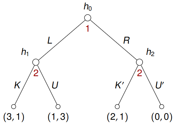
Find all pure strategies of both players – for player 2, there are 4 strategies ($KK', KU', UK', UU'$ with the usual notation $h_1 \mapsto K, h_2 \mapsto K'$ for $KK'$). Is any strategy (strictly, weakly, very weakly) dominant? For player 2, $UK'$ is weakly dominant. Is any strategy (strictly, weakly, very weakly) dominated? Is any strategy never best response? Are there Nash equilibria in pure strategies?

Table for extensive-form game
	$KK'$	$KU'$	$UK'$	$UU'$
$L$	$(3,1)$	$(3,1)$	$(1,3)$	$(1,3)$
$R$	$(2,1)$	$(0,0)$	$(2,1)$	$(0,0)$

Writing it in a table converts it into a strategic-form game. As such, it is much easier to see Nash equilibria $R, UK'$ and $L, UU'$. When we examine $(L, UU')$, we obtain:

player 2 threats to play $U'$ in $h_2$,
as a result, player 1 plays $L$,
player 2 reacts to $L$ by playing the best response, i.e. $U$.

However, the threat is not credible, once a play reaches $h_2$, a rational player 2 chooses $K'$. Now examine $(R, UK')$, which is sensible in the following sense

player 2 plays the best response in both $h_1$ and $h_2$,
player 1 plays the “best response” in $h_0$ assuming that player 2 will play his best responses in the future.

This equilibrium is called subgame perfect.

Given $h \in \mathcal{H}$, we denote $\mathcal{H}^h$ the set of all nodes reachable from $h$.

Definition 5.3 (Subgame) A subgame $G^h$ of $G$ rooted at $h \in \mathcal{H}$ is the restriction of $G$ to nodes reachable from $h$ in the game tree. More precisely, \[ G^h = (N,A,H^h, \chi^h, \rho^h, \pi^h, h, \boldsymbol{u}^h) \] where $H^h = H \cap \mathcal{H}^h$, $Z^h = Z \cap \mathcal{H}^h$, $\chi^h$ and $\rho^h$ are restrictions of $\chi$ and $\rho$ to $H^h$, respectively. Moreover

$\pi^h$ is defined for $h' \in H^h$ and $a \in \chi^h(h')$ by $\pi^h(h', a) = \pi(h', a)$;
each $u_i^h$ is a restriction of $u_i$ to $Z^h$.

Tip

Given a function $f: A \to B$ and $C \subseteq A$, a restriction of $f$ to $C$ is a function $g : C \to B$ such that $g(x) = f(x)$ for all $x \in C$

Definition 5.4 (Subgame Perfect Equilibrium) A subgame perfect equilibrium (SPE) in pure strategies is a pure strategy profile $\boldsymbol{s} \in S$ such that for any subgame $G^h$ of $G$, the restriction of $\boldsymbol{s}$ to $H^h$ is a Nash equilibrium in pure strategies in $G^h$.

Note

A restriction of $\boldsymbol{s} = (s_1, \dots, s_n) \in S$ to $H^h$ is a strategy profile $\boldsymbol{s}^h = (s_1^h, \dots, s_n^h)$ where $s_i^h(h') = s_i(h')$ for all $i \in N$ and all $h' \in H_i \cap H^h$.

Example 5.8 Recall the Stackelberg competition Example 5.3. Player 1 chooses $q_1$, and we know that the best response of player 2 is $q_2 = (\theta- q_1) /2$ where $\theta= \kappa - c$. Then \[ u_1(z^{q_1, q_2}) = q_1(\theta- q_1 - \theta/2 - q_1/2) = (\theta/2)q_1 - q_1^2 /2 \] which is maximized by $q_1 = \theta/2$, giving $q_2 = \theta/4$. So \[ u_1(z^{q_1, q_2}) = \theta^2/8, \qquad u_2(z^{q_1, q_2}) = \theta^2/16 \]

Note that firm 1 has an advantage as a leader.

5.4 Backward Induction

An algorithm for computing SPE for finite perfect-information extensive-form games.

Definition 5.5 (Backward Induction) We inductively “attach” to every node $h$ a pure strategy profile $\boldsymbol{s}^h = (s_1^h, \dots, s_n^h)$ in $G^h$, together with a vector of expected payoffs $\boldsymbol{u}(h) = (u_1(h), \dots, u_n(h))$.

Initially - Attach to each terminal node $z \in Z$ the empty profile $\boldsymbol{s}^z = (\emptyset, \dots, \emptyset)$ and the payoff vector $\boldsymbol{u}(z) = (u_1(z), \dots, u_n(z))$.
While (there is an unattached node $h$ with all children attached):
1. Let $K$ be the set of all children of $h$;
2. Let \[ h_{\max} \in \mathop{\mathrm{argmax}}_{h' \in K} \, u_{\rho(h)}(h'); \]
3. Attach to $h$ a strategy profile $\boldsymbol{s}^h$ where
  - $\pi(h, s^h_{\rho(h)}(h)) = h_{\max}$;
  - for all $i \in N$ and all $h' \in H^h_i \setminus \left\{h\right\}$ (at the same time $h' \in H^{\bar h} \cap H_i$ for an appropriate $\bar h \in K$) define $s_i^h(h') = s_i^{\bar h}(h')$ where $\bar h \in K$;
4. Attach to $h$ the vector of expected payoffs $\boldsymbol{u}(h) := \boldsymbol{u}(h_{\max})$.

Example 5.9 Recall the game

Then clearly \[ \boldsymbol{s}^{z_1} = \boldsymbol{s}^{z_2} = \boldsymbol{s}^{z_3} = \boldsymbol{s}^{z_4} = (\emptyset, \emptyset). \]

Now for $h_1$, where the second player makes a choice (and his better choice is $U$ getting him $(1,3)$), we get \[ \boldsymbol{s}^{h_1} = (s_1^{h_1}, s_2^{h_2}) = (\emptyset, \left\{(h_1, U)\right\}) \implies \boldsymbol{u}(h_1) = (1,3) \] and similarly \[ \boldsymbol{s}^{h_2} = (\overbrace{\emptyset}^{s_1^{h_2}}, \overbrace{\left\{(h_2, K')\right\}}^{s_2^{h_2}}) \implies \boldsymbol{u}(h_2) = (2,1). \]

Finally considering $h_0$, where $\rho(h_0) = 1$, we see that \[ \boldsymbol{s}^{h_0} = \left( \left\{(h_0, R)\right\}, \left\{(h_1, U), (h_2, K')\right\} \right) \implies \boldsymbol{u}(h_0) = (2,1). \]

Theorem 5.1 For every finite perfect-information extensive-form game and for each node $h$ the attached $\boldsymbol{s}^h$ is a SPE and the attached vector $\boldsymbol{u}(h)$ satisfies $\boldsymbol{u}(h) = \boldsymbol{u}(\boldsymbol{s}^h) = (u_1(\boldsymbol{s}^h), \dots, u_n(\boldsymbol{s}^h))$.

Proof. We will lead the proof by induction. In any terminal node $z$ no player has any choice, thus empty strategies make a SPE with payoffs $\boldsymbol{u}(z)$.

Now assume that $h$ is being processed in the while loop. Denote by $\bar{\boldsymbol{s}}^h$ a profile obtained from $\boldsymbol{s}^h$ by changing the strategy of player $i$. We split the situation into two different cases. First, we assume that player $i$ does not control $h$, i.e. $\rho(h) \neq i$. Let $\bar{\boldsymbol{s}}^{h_{\max}}$ be the restriction of $\bar{\boldsymbol{s}}^h$ to the subgame rooted in $h_{\max}$, see Figure 5.1.

Figure 5.1: Case when player $i$ does not control $h$

Here hₘ denotes $h_{\max}$ and sᵐ, and s̄ᵐ, the profiles $\boldsymbol{s}^{h_{\max}}$, and $\bar {\boldsymbol{s}}^{h_{\max}}$ respectively. By induction we then get \[ u_i(\boldsymbol{s}^h) = u_i(\boldsymbol{s}^{h_{\max}}) \geq u_i (\bar{\boldsymbol{s}}^{h_{\max}}) = u_i(\bar{\boldsymbol{s}}^h). \]

Second, we assume $i = \rho(h)$ and denote by $\bar h = \bar s^h_{\rho(h)}$. Let $\bar{\boldsymbol{s}}^{\bar h}$ be the restriction of $\bar{\boldsymbol{s}}^h$ to the subgame rooted in $\bar h$. Then also, see Figure 5.2, \[ u_i(\bar{\boldsymbol{s}}^h) = u_i(\bar{\boldsymbol{s}}^{\bar h}) \leq u_i(\boldsymbol{s}^{\bar h}) \leq u_i(\boldsymbol{s}^{h_{\max}}) = u_i(\boldsymbol{s}^h). \tag{5.1}\]

Figure 5.2: Case when player $i$ controls $h$, sᵇ denotes $\boldsymbol{s}^{\bar h}$ and s̄ᵇ profile $\bar{\boldsymbol{s}}^{\bar h}$

The first inequality in (5.1) is true by the induction step and the second holds by the definition of $h_{\max}$. In both cases the deviation of player $i$ leads to a smaller or equal playoff. Hence $\boldsymbol{u}(\boldsymbol{s}^h) = \boldsymbol{u}(\boldsymbol{s}^{h_{\max}}) = \boldsymbol{u}(h_{\max}) = \boldsymbol{u}(h)$. This concludes the proof.

Example 5.10 (Chess – continued) Recall that in the model of chess, the payoffs were from $\left\{1, 0, -1\right\}$ and $u_1 = - u_2$ (i.e. chess is a zero-sum game). By Theorem 5.1, there is a SPE in pure strategies $\boldsymbol{s}^* = (s_1^*, s_2^*)$. However, then one of the following holds:

white has a winning strategy (if $u_1(\boldsymbol{s}^*) = 1$ and thus $u_2(\boldsymbol{s}^*) = -1$);
black has a winning strategy (if $u_2(\boldsymbol{s}^*) = 1$ and thus $u_1(\boldsymbol{s}^*) = -1$);
both players have strategies to force draw (if $u_1(\boldsymbol{s}^*) = 0$ and thus $u_2(\boldsymbol{s}^*) = 0$).

Now the question arises what is the right answer, but, in truth, nobody knows yet, as the tree of the game is too big. Even simplifying to trees only about 200 edges deep and with approximately 5 moves per node on average, we get a total count of $5^{200}$ nodes!

Recall that in the second step of Definition 5.5, the algorithm may choose an arbitrary $h_{\max} \in \mathop{\mathrm{argmax}}_{h' \in K} u_{\rho(h)}(h')$ and always obtain a SPE. Thus to compute all SPEs, the algorithm may systematically search through all possible choices of $h_{\max}$ throughout the induction.

Also one can realize that backward induction, see Definition 5.5, is too inefficient, as it unnecessarily searches through the whole tree. There are better methods mitigating this problem, e.g. $\alpha$-$\beta$-pruning.

5.4.1 Criticism of Subgame Perfect Equilibria

Example 5.11 Consider the following game, called centipede:

By backward induction, we can obtain that the SPE in pure strategies is $(DDD, DD)$ – this should be at least a little bit weird. There are serious issues here:

In a laboratory setting, people usually play $A$ for several steps.
There is a theoretical problem: Imagine, that you are player 2. What would you do when player 1 chooses $A$ in the first step? The SPE analysis says that you should go down, but the same analysis also says that the situation you are in cannot appear :-)

	\(KK'\)	\(KU'\)	\(UK'\)	\(UU'\)
\(L\)	\((3,1)\)	\((3,1)\)	\((1,3)\)	\((1,3)\)
\(R\)	\((2,1)\)	\((0,0)\)	\((2,1)\)	\((0,0)\)