7 Imperfect-Information Games

7.1 Introduction

Is it possible to model Matching pennies using extensive-form games?

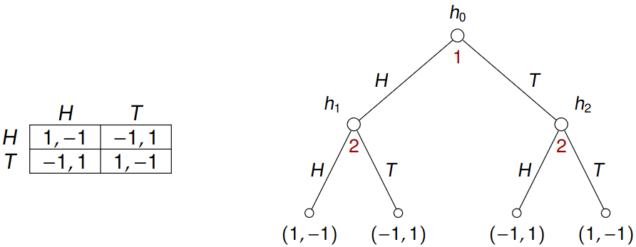
The problem is that player 2 is “perfectly” informed about the choice of player 1. In particular, there are pure Nash equilibria \((H, TH)\) and \((T, TH)\) in the extensive-form game as opposed to the strategic-form, where there is none. Reversing the order of players does not help.

Thus, we need to extend the formalism to be able to hide some information about previous moves.

Matching pennies can be modeled using an imperfect-information extensive-form game:

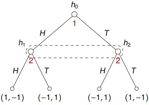
Here \(h_1\) and \(h_2\) belong to the same information set of player 2. As a result, player 2 is not able to distinguish between \(h_1\) and \(h_2\). So even though players do not move simultaneously, the information player 2 has about the current situation is the same as in the simultaneous case

Note

There must be the same set of actions from all nodes of the information set. Otherwise, the player would be able to deduce information about the current state.

Caution

No history is inherently encoded in the game (so if we want to provide past moves of the player as input for his decision process, we have to encode it in the notes themselves). Otherwise, the player could be able to deduce more information about the current state of the game.

7.2 Definition of Imperfect-Information Game

Definition 7.1 An imperfect-information extensive-form game is a tuple \({G}_{\mathrm{imp}} = ({G}_{\mathrm{perf}}, \boldsymbol{I})\) where

\({G}_{\mathrm{perf}} = (N,A,H,Z, \chi, \rho, \pi, h_0, \boldsymbol{u})\) is a perfect-information extensive-form game (called the underlying game),
\(\boldsymbol{I} = (I_1, \dots, I_n)\) where for each \(i \in N = \left\{1, \dots, n\right\}\) \[ I_i = \left\{I_{i,1}, \dots, I_{i,k_i}\right\} \] is a collection of information sets for player \(i\) that satisfies
- \(\bigcup_{j = 1}^{k_i} I_{i,j} = H_i\) and \(I_{i,j} \cap I_{i,k} = \emptyset\) for \(j \neq k\) (i.e. \(I_i\) is a partition of \(H_i\), see Definition 5.1);
- for all \(h, h' \in I_{i,j}\), we have \(\rho(h) = \rho(h')\) and \(\chi(h) = \chi(h')\) (i.e., nodes from the same information set are owned by the same player and have the same sets of enabled actions).

Given \(h \in H\), we denote by \(I(h)\) the information set \(I_{i,j}\) containing \(h\). Also, given an information set \(I_{i,j}\), we denote by \(\chi(I_{i,j})\) the of all action enabled in some (and hence all, per Definition 7.1) nodes of \(I_{i,j}\).

Now we define the set of pure, mixed, and behavioral strategies in \({G}_{\mathrm{imp}}\) as subsets of pure, mixed, and behavioral strategies, resp., in \({G}_{\mathrm{perf}}\) that respect the information sets. Let \({G}_{\mathrm{imp}} = ({G}_{\mathrm{perf}}, \boldsymbol{I})\) be an imperfect-information extensive-form game where \({G}_{\mathrm{perf}} = (N,A,H,Z, \chi, \rho, \pi, h_0, \boldsymbol{u})\).

Definition 7.2 A pure strategy of player \(i\) in \({G}_{\mathrm{imp}}\) is a pure strategy \(s_i\) in \({G}_{\mathrm{perf}}\) such that for all \(j = 1, \dots, k\) and all \(h, h' \in I_{i,j}\) holds \(s_i(h) = s_i(h')\).

Tip

Note that each \(s_i\) can also be seen as a function \(s_i : I_i \to A\) such that for every \(I_{i,j} \in I_i\) we have that \(s_i(I_{i,j}) \in \chi(I_{i,j})\).

As before, we denote by \(S_i\) the set of all pure strategies of player \(i\) in \({G}_{\mathrm{imp}}\), and by \(S = S_1 \times \dots \times S_n\) the set of all pure strategy profiles. As in the perfect-information case we have a corresponding strategic-form game \(\bar {G}_{\mathrm{imp}} = (N, (S_i)_{i \in N}, (u_i)_{i \in N})\).

7.3 Examples

Example 7.1 (Matching Pennies) Recall the game of matching pennies:

Here \(I_1 = \left\{I_{1,1}\right\}\) where \(I_{1,1} = \left\{h_0\right\}\) and \(I_2 = \left\{I_{2,1}\right\}\) where \(I_{2,1} = \left\{h_1, h_2\right\}\). An example of pure strategies might be:

\(s_1(I_{1,1}) = H\) which describes strategy \(s_1(h_0) = H\);
\(s_2(I_{2,1}) = T\) which describes strategy \(s_2(h_1) = s_2(h_2) = T\) (it is also sufficient to specify \(s_2(h_1) = T\) since then by definition \(s_2(h_2) = T\)).

Thus we really only have strategies \(H,T\) for player 1 and \(H,T\) for player 2.

Example 7.2 Consider now a game given by:

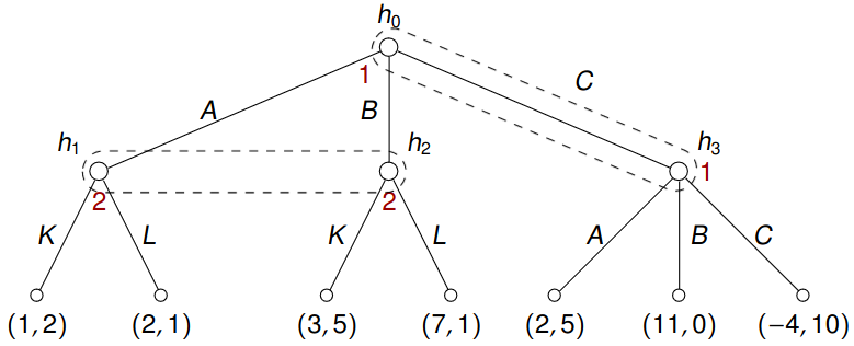
Note that \(I_1 = \left\{I_{1,1}\right\}\) where \(I_{1,1} = \left\{h_0, h_3\right\}\) and that \(I_2 = \left\{I_{2,1}\right\}\) where \(I_{2,1} = \left\{h_1, h_2\right\}\). The pure strategies in this example are

\(s(I_{1,1}) \in \left\{A, B, C\right\}\) for player 1;
\(s(I_{2,1}) \in \left\{K, L\right\}\) for player 2.

Playing \(A\) or \(B\) from \(h_3\) is unreachable (or illegal/unfeasible) in this game with pure and mixed strategies.

7.4 Subgame-perfect Equilibria in Imperfect-Information Games

Now we shall turn our attention to the following game: h₂

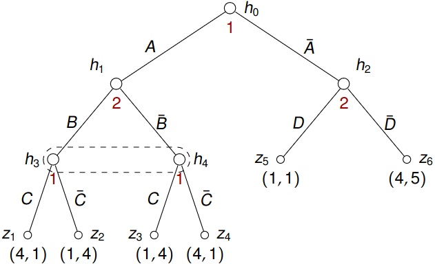
What do we designate as subgames to allow the backward induction, with which we could calculate subgame-perfect equilibria (or more precisely their equivalents here)? Only subtrees rooted in \(h_1, h_2\), and \(h_0\) (together will all subtrees rooted in terminal nodes) seem reasonable. Note that subtrees rooted in \(h_3\) and \(h_4\) cannot be considered as “independent” subgames because their individual solution cannot be combined to a single best response in the information set \(\left\{h_3, h_4\right\}\).

Let \({G}_{\mathrm{imp}} = ({G}_{\mathrm{perf}}, \boldsymbol{I})\) be an imperfect-information extensive-form game where \({G}_{\mathrm{perf}} = (N,A,H,Z, \chi, \rho, \pi, h_0, \boldsymbol{u})\) is the underlying perfect-information extensive-form game.

Let us denote by \({H}_{\mathrm{proper}}\) the set of all \(h \in H\) that satisfy the following:
For every \(h'\) reachable from \(h\) (that includes the node \(h\) itself), we have that either all nodes of \(I(h')\) are reachable from \(h\), or no node of \(I(h')\) is reachable from \(h\).

Note

Intuitively, \(h \in {H}_{\mathrm{proper}}\) iff every information set \(I_{i,j}\) is either completely contained in the subtree rooted in \(h\), or no node of \(I_{i,j}\) is contained in the subtree.

Definition 7.3 For every \(h \in {H}_{\mathrm{proper}}\) we define a subgame \({G}_{\mathrm{imp}}^h\) to be the imperfect information game \(({G}_{\mathrm{perf}}^h, \boldsymbol{I}^h)\) where \(\boldsymbol{I}^h\) is the restriction of \(\boldsymbol{I}\) to \(H^h\).

Tip

Note that as subgames of \({G}_{\mathrm{imp}}\) we consider only subgames of \({G}_{\mathrm{perf}}\) that respect the information sets, i.e. are rooted in nodes of \({H}_{\mathrm{proper}}\).

Definition 7.4 A strategy profile \(\boldsymbol{s} \in S\) is a subgame-perfect equilibrium (SPE) if \(\boldsymbol{s}^h\) is a Nash equilibrium in every subgame \({G}_{\mathrm{imp}}^h\) of \({G}_{\mathrm{imp}}\) (here \(h \in {H}_{\mathrm{proper}}\)).

Important

The way we generalized subgame-perfect equilibria is not the only one. But others are more complicated and use some kind of randomization.

7.4.1 Backwards Induction

Now we can generalize the backward induction to imperfect-information games, as we hypothesized, along the following lines:

As in the perfect-information case, the goal is to label each node \(h \in {H}_{\mathrm{proper}} \cup Z\) with a SPE \(\boldsymbol{s}^h\) and a vector of payoffs \(\boldsymbol{u}(h) = (u_1(h), \dots, u_n(h))\) for individual players according to \(\boldsymbol{s}^h\).
Starting with terminal nodes, the labeling proceeds bottom up. Terminal nodes are labeled similarly as in the perfect-information case.
Consider \(h \in {H}_{\mathrm{proper}}\), let \(K\) be the set of all \(h' \in \left( {H}_{\mathrm{proper}} \cup Z \right) \setminus \left\{h\right\}\) that are \(h\)’s closest descendants out of \({H}_{\mathrm{proper}} \cup Z\), i.e. \(h' \in K \iff h' \neq h\) is reachable from \(h\) and the unique path from \(h\) to \(h'\) visits only nodes of \(\mathcal{H} \setminus {H}_{\mathrm{proper}}\) (except the first and the last node). For every \(h' \in K\) we already computed a SPE \(\boldsymbol{s}^{h'}\) in \({G}_{\mathrm{imp}}^{h'}\) and the vector of corresponding payoffs \(\boldsymbol{u}(h')\).
Now consider all nodes of \(K\) as terminal nodes where each \(h' \in K\) has payoffs \(\boldsymbol{u}(h')\). This gives a new game in which we compute an equilibrium \(\bar{\boldsymbol{s}}^h\) together with the vector \(\boldsymbol{u}(h)\). The equilibrium \(\boldsymbol{s}^h\) is then obtained by “concatenating” \(\bar{\boldsymbol{s}}^h\) with all \(\boldsymbol{s}^{h'}\), here \(h' \in K\), in the subgames \({G}_{\mathrm{imp}}^{h'}\) of \({G}_{\mathrm{imp}}^h\).

7.4.2 Examples

Example 7.3 (Mutually Assured Destruction) This example is an adaptation of the Analysis of Cuban Missile Crisis of 1962 (as described in Games for Business and Economics by R. Gardner):

The crisis started with the United States’ discovery of Soviet nuclear missiles in Cuba.
The USSR then backed down, agreeing to remove the missiles from Cuba, which suggests that US had a credible threat “if you don’t back off we both pay dearly”.

But could this be a credible threat? We shall model this situation as an extensive-form game:

First, player 1 (US) chooses to either ignore the incident (\(I\)), resulting in maintenance of status quo (payoffs \((0,0)\)), or escalate the situation \((E)\).
Following escalation by player 1, player 2 (USSR) can back down (\(B\)), causing it to lose face (payoffs \((10, -10)\)), or it can choose to proceed to a nuclear confrontation (\(N\)).
Upon this choice, the players play a simultaneous-move game in which they can either retreat (\(R\)), or choose doomsday (\(D\)).
- If both retreat, the payoffs are \((-5, 5)\), a small loss due to a mobilization process.
- If either of them chooses doomsday, then the world destructs and payoffs are \((-100, -100)\).

This game can be re-written into the following tree:

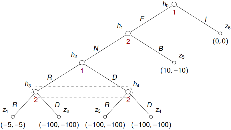
First and foremost, one can solve \({G}_{\mathrm{imp}}^{h_2}\) (a strategic-form game). Then \({G}_{\mathrm{imp}}^{h_1}\) by solving a game rooted in \(h_1\) with terminal nodes \(h_2\) and \(z_5\) (payoffs in \(h_2\) correspond to an equilibrium in \({G}_{\mathrm{imp}}^{h_2}\)). Finally, one solves \({G}_{\mathrm{imp}}\) by solving a game rooted in \(h_0\) with terminal nodes \(h_1\) and \(z_6\) (payoffs in \(h_1\) have been computed in the previous step). This produces 2 SPEs \(\boldsymbol{s}_1 = ((I, R), (N, R))\) and \(\boldsymbol{s}_2 = ((E, D), (B, D))\).

7.5 Mixed and Behavioral Strategies

Definition 7.5 A mixed strategy \(\sigma_i\) of player \(i\) in \({G}_{\mathrm{imp}}\) is a mixed strategy of player \(i\) in the corresponding strategic-form game \({\bar G}_{\mathrm{imp}} = (N, (S_i)_{i \in N}, u_i)\). As before, we denote by \(\Sigma_i\) the set of all mixed strategies of player \(i\).

Do not forget that in the corresponding game \({\bar G}_{\mathrm{imp}}\) any strategy \(s_i \in S_i\) iff \(s_i\) is a pure strategy that assigns the same action to all nodes of every information set. Hence each \(s_i \in S_i\) can be seen as a function \(s_i : I_i \to A\).

Definition 7.6 A behavioral strategy of player \(i\) in \({G}_{\mathrm{imp}}\) is a behavioral strategy \(\beta_i\) in \({G}_{\mathrm{perf}}\) such that for all \(j = 1, \dots, k_i\) and all \(h, h' \in I_{i,j} : \beta_i(h) = \beta_i(h')\) .

Here each \(\beta_i\) can be seen as a function \(\beta_i : I_i \to \Delta(A)\) such that for all \(I_{i,j} \in I_i\) we have \(\mathrm{supp}\left( \beta_i(I_{i,j}) \right) \subseteq \chi(I_{i,j})\).

Note

For behavioral strategy, the distribution of probabilities always stays the same across the information set, unlike in the mixed strategy case, when the randomly selected pure strategy stays the same across the strategy set

Example 7.4 Consider a game

One mixed strategy is \[ \left( \frac 1 2 (AC), 0(BD), 0(BC), \frac 1 2 (BD) \right), \] but this mixed strategy cannot be expressed using behavioral strategies.

Note

Here \(ACC, ACD, ADC, ADD, BCC, BCD, BDC, BDD\) are pure strategies in perfect information. The information set \(\left\{h_1, h_1'\right\}\) restricts us to \(AC, BC, AD, BD\), where the second strategy refers to a strategy on the information set.

Also, notice that mixed strategies don’t really make sense in real life too much.

7.6 Perfect Recall

Example 7.5 Consider the following game of the so-called absent-minded driver:

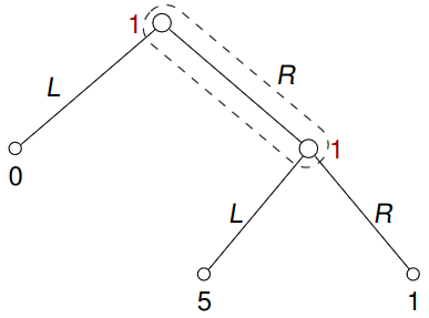
Note that there is only one player: A driver who has to take a turn at a particular junction. There are two identical junctions, the first one leads to a wrong neighborhood where the driver gets completely lost (payoff 0), and the second one leads home (payoff 5). If the driver misses both, there is a long way home (payoff 1). The problem is that after missing the first turn, the driver forgets that he missed the turn.

Notice that the behavioral strategy \(\beta_1(I_{1,1})(L) = \frac 1 2\) has the expected payoff \(\frac 3 2\). Also, it can be shown that no mixed strategy gives a larger payoff than 1 since no pure strategy ever reaches the terminal node with a payoff 5.

We say that player \(i\) has perfect recall in \({G}_{\mathrm{imp}}\) if the following holds:

Every information set of player \(i\) (i.e., his own) intersects every path from the root \(h_0\) to a terminal node at most once (so no absent-minded driver situation occurs, see Example 7.5).
Every two paths from the root that end in the same information set of player \(i\)
- pass through the same information sets of player \(i\),
- and in the same order,
- and in every such information set the two paths choose the same actions.

Warning

These two paths, however, may pass through different information sets of other players and other players may choose different actions along each of the paths!

I.e. each information set \(J\) of player \(i\) determines the sequence of information sets of player \(i\) and actions taken by player \(i\) along any path reaching \(J\).

Theorem 7.1 (Kuhn, 1953) Assuming perfect recall, every mixed strategy can be translated to a behavioral strategy (and vice versa) so that the payoff for the resulting strategy is the same in any mixed profile.